SurfCalc User Guide¶

Welcome to SurfCalc, an optomechanical analysis suite that turns structural FEA results into optical surface and wavefront performance data. This guide provides an end-to-end overview of the application interface, functionality, layout options, and standard analysis workflows.

1. Application Overview¶

SurfCalc is designed to analyze optomechanical surface deformations of high-precision mirrors (such as telescope primary/secondary mirrors) using finite element analysis (FEA) results or coordinate measurement data. The application is divided into five main workspaces:

1. Surface Deformation Module: Imports mesh displacement data, fits Zernike polynomials (or other bases), removes Rigid Body Motion (RBM), and performs coordinate unit conversions.
2. Load Case Combination Module: Combines several separate FEA load cases (gravity, thermal soak, wind, ...) into one deformation field by signed superposition or RSS envelope, feeding one or more Surface Deformation fits and/or an Active Optics target.
3. Influence Matrix Generator Module: Decouples multi-actuator load cases into independent solver decks, generates an external batch runner, projects completed FEA displacements onto local surface normals, and compiles the system influence matrix.
4. Bending Modes Module: Extracts a normal-modes basis directly from an FEA modal analysis (Abaqus/Ansys/Nastran) or a hand-built CSV, feeding one or more Surface Deformation fits with a live-updating link.
5. Active Optics Correction Module: Executes bounded or unconstrained active optics correction solvers, evaluates corrected RMS surface quality, maps actuator load layouts, and exports force commands.

2. Global Interface & Sidebar¶

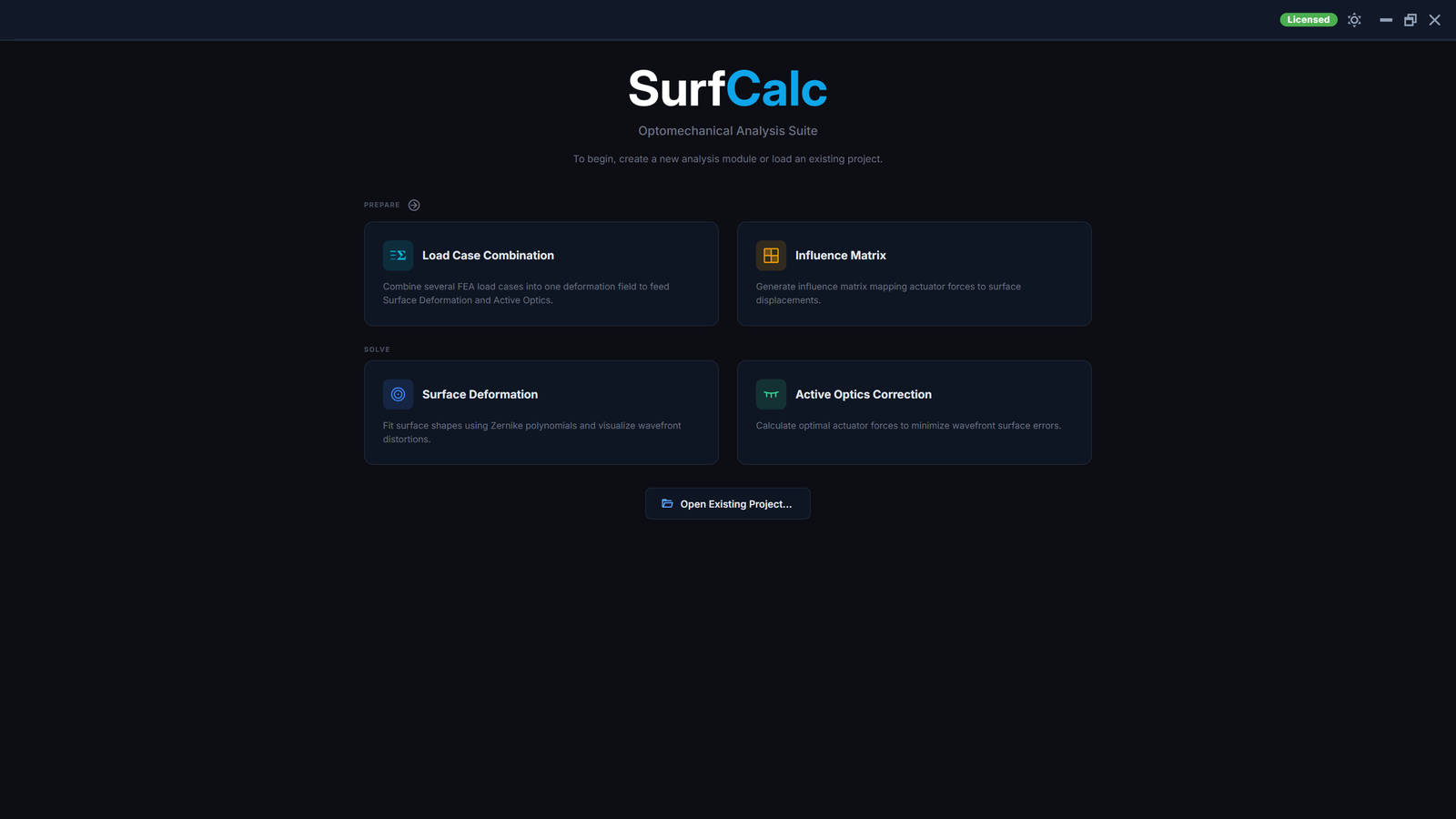
Project Explorer & Welcome Page¶

• Welcome Page: On startup or when creating a new project, SurfCalc displays a clean Welcome Page dashboard. You can click on cards to instantly initialize analysis modules.
• Dynamic Sidebar Explorer: When modules are active, the sidebar becomes visible. It displays a hierarchical project tree representing active modules.
• Dynamic Naming: The root of the Project Explorer tree displays the actual file name of the currently saved project (e.g. primary_mirror.surfcalc). If the project has not been saved, it defaults to New Project.
• Imported Units Display: For each active module, the Project Explorer tree dynamically displays an auto-expanded child node representing the exact imported units for the loaded dataset (e.g., Imported Units: [mm, rad, N]) directly underneath the input file node, providing instant contextual awareness.
• State Preservation Alerts: If you attempt to close the application or open a new file with unsaved changes, SurfCalc will display an alert dialog prompting you to save your work. (Note: These dialogs are automatically bypassed in headless CLI mode).

Color Themes¶

• SurfCalc supports Light Mode and Dark Mode. You can switch themes under preferences.
• Interactive 3D plotters, legends, tables, and 2D graphs dynamically adjust their backgrounds, fonts, and coordinate grids to match the selected theme.
• Viewport Background (Preferences) can be detached from the theme. Leave Override Color Theme off and the 3D viewports follow the app theme as before; switch it on and pick Black or White to pin the 3D background regardless of which theme the rest of the interface is using — useful for producing figures for print or for presenting on a projector. Annotations drawn over the viewport (the scale bar) follow the background you pin, not the theme, so they stay legible either way.

Interactive 3D Plotter Controls & Context Menu¶

SurfCalc provides premium, direct-manipulation interactivity across all of its interactive 3D viewports. Rather than forcing you to navigate away to global settings, you can right-click directly inside any 3D viewport to access a premium, theme-adaptive context menu. The toolbar's Tools menu mirrors the same categories as a second, always-reachable entry point, for when you'd rather not right-click the viewport itself.

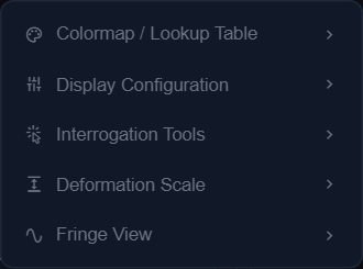
Each category above expands into a flyout submenu of the actual options listed below:

• Change Colormap: Instantly override and update the active colormap locally on that viewport. Choose from a selection of modern palettes: Coolwarm, Jet, Viridis, Plasma, Inferno, Magma, Rainbow, or revert to the Default theme colormap.
• Set Color Limits...: Open a local dialog to customize the exact numerical minimum and maximum scalar bounds for the 3D surface plot's color legend.
• Show Orientation Axes: Toggle the small red/green/blue X/Y/Z triad shown in each viewport's top-right corner (see below).
• Toggle Orthographic / Perspective Projection: Switch the camera projection mode for every viewport.
• Show Scale Bar: Toggle the scale bar in each viewport's bottom-left corner (see below).
• Clip Plane...: Open the Clip Plane dialog (see below).
• Probe Point Value / Measure Distance: Arm one of the two interrogation tools (see below). Selecting an already-active tool switches it back off.
• Deformation Scale: Control how far the displayed surfaces are exaggerated out of plane, plus Show Undeformed Reference and Render Solid Surface (see below).

Each viewport's own toolbar has a separate ORIENT: row with ISO / XY / XZ / YZ / Fit buttons that reorient the camera to a standardized viewpoint:

• ISO — standard isometric 3D perspective.
• XY / XZ / YZ — top, front, and side plan views, looking straight down the third axis. Pressing the same button again flips to that plane's opposite side (e.g. XY twice gives a top-down view, then a bottom-up one) — press ISO first if you want the next press to start from the positive side again.
• Fit — recenters and zooms to fit the model bounds, without changing the current viewing direction.

Alongside them sit the Probe and Measure tools (see below) and a copy button, which screenshots the module's currently visible viewports — stitched side by side in the order they appear on screen — and puts the image on your clipboard, ready to paste into a report or an email.

You can also click directly on the X, Y, or Z label of the corner orientation triad to align that pane to the plane you'd be looking at face-on down that axis (clicking X aligns to the YZ plane, and so on) — clicking the same axis again flips to its opposite side, the same way the toolbar buttons do. With Sync Views on, the other viewports in that module follow; with it off, only the clicked viewport reorients.

Deformation Scale¶

Surface displacements are typically microns or nanometres on a mirror hundreds of millimetres across, so every 3D viewport adds them, exaggerated, on top of the mesh's own Z coordinate — otherwise the wrinkles would be invisible on the figure. The undeformed surface shape is always kept; only the selected deformation (normal displacement, local-Z sag, mode shape, or influence function) is scaled. The Deformation Scale section of the right-click menu is where that exaggeration is controlled, and it applies to Surface Deformation, Influence Matrix, Active Optics Correction, Load Case Combination, and Bending Modes.

• Auto Deformation Scale (on by default) sizes each surface so its peak-to-valley deformation reaches 5% of the model's own width, whatever the physical magnitude. The factor actually being applied is reported underneath as Current: N×. Switching it off reveals a Scale Factor field, pre-filled with the factor Auto had just been using — so the view doesn't jump — which you can then set to any exaggeration you want. A custom factor multiplies the displayed displacement values directly, so it depends on the display units currently selected.
• Auto-Equalize Displacements (on by default) makes every surface in the module reach the same peak deformation height rather than being scaled independently: the Original/Fit/Residual panes in Surface Deformation, the Target/Fit/Residual panes in Active Optics Correction, and the actuators you scrub through in the Influence Matrix inspector. This matters most with a custom Scale Factor — a well-corrected residual is often orders of magnitude smaller than the target it came from, and would otherwise show only the undeformed figure with no visible residual wrinkles. Turn it off when you want the relative magnitudes themselves to be visible.

The exaggeration is a display convention only — it never affects fitted coefficients, RMS/PV values, forces, or anything written to an export.

One display is deliberately exempt: the Influence Matrix Post-processor's node-set and load-step previews always show the model undeformed, since their purpose is to confirm the geometry that came out of the FE deck.

Show Undeformed Reference, Clip Plane & Render Solid Surface¶

Three further options live in the same right-click Deformation Scale category — and are mirrored as a second entry point under the toolbar's Tools > Deformation Scale menu — for Surface Deformation, Influence Matrix, Active Optics Correction, and Bending Modes; Render Solid Surface additionally covers Load Case Combination (Show Undeformed Reference and Clip Plane don't, since Load Cases' combined-result viewport has no single deformed-vs-undeformed pane to overlay or cut).

• Show Undeformed Reference superimposes the true, unscaled surface as a translucent ghost — Solid or Wireframe — underneath the exaggerated deformed one, so the Deformation Scale exaggeration reads against a real size reference instead of floating in isolation.
• Clip Plane... opens a small, draggable, non-modal dialog — move it aside, or keep adjusting the cut while you rotate the model; it never closes on its own — to hide part of the mesh on one side of a plane: pick an X / Y / Z / Custom normal, drag or type the cut Position as a percentage across the model's bounds, and Invert Side to flip which half is hidden.
• Render Solid Surface extrudes the displayed shell into a solid body by a real physical Thickness, mimicking how FEA post-processors render shell elements with their real thickness. The Thickness comes from the module's selected Optical Surface (see the Optical Surface Library section below) — with none selected, or none with a Thickness set, the toggle safely falls back to the normal thin shell and logs a one-time console reminder rather than failing silently. Three further controls appear once it's on:
  • Mid-Surface (both directions) treats the displayed mesh as the physical mid-plane and extrudes half the thickness to each side, the usual FEA convention (nodes on the neutral surface, shell extends evenly either side of it). Off by default, which instead extrudes the full thickness to one side only.
  • Flip Direction (hidden while Mid-Surface is on, since it has no visible effect there — splitting the thickness evenly either side looks the same regardless of which side is called "front") reverses which side the material is added to. The default side is a geometric guess based on the mesh's own geometry, with no knowledge of which face is a real mirror's optically active surface — flip it if the solid comes out the wrong way.
  • Thickness Scale — True Thickness (no scaling) (default) renders the mirror's real, physical thickness at the model's real geometric scale. Custom Scale (×) instead multiplies it by a typed factor, for the rare case you specifically want the solid's apparent thickness to track a pane's own Deformation Scale exaggeration — read that pane's Current: N× readout above and type it in.

Enabling Render Solid Surface together with Clip Plane cuts a real cross-section through the solid's thickness, rather than a flat clipped shell.

Scale Bar¶

Turning on Show Scale Bar (right-click menu, or Preferences) puts a short labelled ruler along the bottom of every 3D viewport, centred, in the same spirit as the scale indicator in Fluent or CFD-Post. The label always reads a round number (1, 2 or 5 followed by zeros — 20 mm, 50 mm, 1 m …) and the line is drawn at exactly that length on screen, so you can eyeball model dimensions by comparison without measuring anything.

It updates live as you zoom and rotate, and each pane has its own — panes framed differently show different scales. A pane that has nothing loaded yet shows no bar; it appears as soon as there is real geometry to measure against.

The label uses your selected Display Unit (Units menu, or Preferences > Display Units), so it agrees with the scalar legend and the probe readout. That unit is chosen for displacements, though, and won't always suit geometry — a 200 mm mirror in nanometres would read "50000000 nm" — so when the selected unit can't express the length readably the bar falls back to the nearest one that can. Selecting waves likewise falls back, since it measures wavefront error rather than distance.

Probing and Measuring¶

Two interrogation tools are available: from the Probe and Measure buttons in each viewport toolbar (next to the ORIENT row), or from the viewport right-click menu. Both places drive the same setting; the toolbar buttons additionally light up while their tool is armed, and the cursor becomes a crosshair over the viewport, so you can always see that the next click will take a reading.

Only one tool can be armed at a time, since both consume your click on the geometry. Clicking an armed tool's button again switches it off. While either is armed, a readout card appears in the bottom-right corner of the window and names the pane the reading came from; close the card (or switch the tool off) to go back to normal interaction.

• Probe Point Value — click anywhere on the surface to read out that location's coordinates and the scalar value plotted there, in the same display units as the pane's color legend. The click snaps to the nearest mesh node, so the number you get is a real solver result rather than an interpolated one — and a small marker is drawn at that node, so you can see exactly which point the reading came from. The marker is sized from the spacing between that node and its neighbours, so it marks one node rather than covering a patch of them, however finely the model is meshed.
• Measure Distance — click two points on the same pane. The card reports both endpoints, the ΔX/ΔY/ΔZ components, the straight-line distance and the in-plane (XY) distance, and the measured segment is drawn into the viewport so you can see what you measured. Its endpoint markers are sized the same way the probe's is — from the local mesh spacing at each clicked node, not from how far apart the two points happen to be — so they stay legibly node-sized whether you measure between two neighbouring nodes or across the whole model. A third click starts a new measurement.

Both tools report scene coordinates, in your selected Display Unit with the same readability fallback the scale bar uses — so a distance you measure and the scale bar you compare it against always read in the same unit. Each reading picks one unit for all of its rows, so the numbers in a card stay directly comparable. X and Y are always true model coordinates; Z is the undeformed mesh coordinate plus the exaggerated deformation in any pane that has a deformation scale factor applied, so use the probed Value — not Z — as the physical displacement there. The measurement markers are cleared whenever the pane's geometry is rebuilt.

Dynamic Global Preferences¶

The global Preferences dialog (accessible under the File menu or Toolbar) allows configuring the default color maps, styling preferences, and theme choices. The dialog automatically detects which workspace module is currently active:

• If you open Preferences while active on the Influence Matrix Generator, the dialog dynamically re-labels options to display "Influence Matrix Colormap:" for clarity.
• Significant Figures: Controls how many significant digits are shown everywhere a numeric value is displayed — the 3D viewport's scalar-bar legend, PV/RMS and Zernike coefficient tables, RBM translation/rotation readouts, and chart hover tooltips all share this single setting, so precision stays consistent across the app regardless of how many viewport panes are open.

Global Unit System & Bidirectional Sync¶

SurfCalc features a highly robust, unified global unit system. Users can configure the default units for displacements, rotations, and forces at the application-wide level:

• Units Menu: Navigate to Units > Configure Units... on the menu bar to open the Unit Configuration panel. It displays the currently active units: displacement input/output, rotation input/output, and force input/output (e.g. mm, um, rad, deg, N).
• Bidirectional Synchronization: Any unit changes made globally are instantly pushed to the local combo boxes of all active modules (Surface Deformation, Active Correction, etc.). Conversely, modifying a unit locally within any individual tab automatically propagates and updates the global units.
• Real-time Status Bar Updates: The main window's bottom status bar dynamically displays the active units in real time, guaranteeing visual feedback and preventing calculation scale errors.
• Unit Setting Persistence: All configured units (input/import and output/display settings) are automatically saved and persisted in the local application preferences across sessions, ensuring your preferred unit setup is restored on every startup.
• Console Table Unit Filtering: To maintain a clean, uncluttered workspace during active engineering runs, all unit settings tables, logs, and report views rendered inside the bottom collapsible panels filter the columns to display the "Displayed" (output) units only.
• Optical Reference Parameters: When the output/display displacement unit is set to "waves", a nested "Optical Reference Settings" sub-panel dynamically appears inside the Unit Settings panel. This lets you specify the reference wavelength (e.g., in nm, um, mm, m) and choose the Optical Path Difference (OPD) mode—either Surface (1x) for physical surface error, or Reflection (2x) to analyze double-pass wavefront errors. Modifying these values instantly triggers recalculation across active analysis tabs.
• Scientific Toggles for RMS: Standardized formatting toggle checkboxes are available on the analysis panes to instantly switch display formats for RMS values between standard decimal (e.g., 0.00045) and scientific notation (e.g., 4.5e-04).

Optical Surface Library¶

A mirror's prescription — vertex radius of curvature, conic constant, clear aperture, central hole diameter, off-axis decenter, thickness, surface type, material, CTE — can be defined once and referenced from any module, instead of retyping the same numbers in each tab. It drives two independent things: any module's Radial Correction setting (Surface Deformation, Active Optics, Influence Matrix, Load Case Combination), and Render Solid Surface's Thickness (Surface Deformation, Active Optics, Influence Matrix, Load Case Combination, Bending Modes) — see above.

• Pick a surface: every module that can reference one shows an always-visible Optical Surface picker of its own — a dropdown (Manual (typed below) plus every mirror in both libraries) near the top of the sidebar, close to where the module's data is loaded. It's independent of Radial Correction: leave Radial Correction at None and the picker still selects which surface's Thickness is used for Render Solid Surface. Selecting a mirror there also fills in that module's Radial Correction Vertex RoC / Conic Constant fields (in the separate Radial Correction section further down) with the mirror's numbers, read-only, whenever Radial Correction is switched on.
• Manage the library: File > Optical Surfaces... opens the library dialog independent of any module — the same dialog is also reachable via Manage... under any module's Optical Surface picker. It lists two grouped libraries side by side:
  • Project Library — mirrors saved with this project (part of the .surfcalc file). Sharing the project file shares these mirrors with it.
  • App Library — mirrors that persist across every project on this computer (~/.surfcalc_mirrors.json), for a mirror you analyze repeatedly across different projects.
  • Copy to Project / Save to App Library copy a mirror between the two — each copy gets its own identity and can be edited independently afterward; there is no ongoing sync between the copy and the original.
• Editing is explicit, not automatic: typing into a mirror's fields in the library editor only updates a local draft — nothing is written to the record, and no other module sees a change, until you click Save. A Discard button reverts the draft to what's currently saved. Switching to a different row, creating/duplicating a mirror, or closing the dialog while a draft has unsaved changes prompts you to Save & Continue, Discard & Continue, or Cancel first, so a stray edit can't silently overwrite a shared mirror.
• Thickness (m): the substrate/shell thickness, in the same SI-meters convention as the other length fields. Optional — leave it at 0 if you don't use Render Solid Surface. It has no effect on Radial Correction.
• Radial Correction's numbers are a snapshot, not a live link: turning on Radial Correction reads the selected mirror's current RoC/Conic at that moment; a recorded macro or pure-Python statement stores that literal number, not a reference back to the library entry, since a replay elsewhere has no guarantee the same library entry still exists. Render Solid Surface's Thickness, by contrast, is read fresh from the library every time the viewport re-renders (including right after you edit and Save it in the library dialog), so it always reflects the mirror's current saved value.
• Material is recorded for reporting only — SurfCalc consumes already-solved FEA displacement fields; it does not compute thermal loads from a mirror's material. It exists so a report can print the surface's full identity (e.g. "M1 Primary — Zerodur") alongside the prescription. CTE is also available to Load Case Combination's Thermal Free-Growth case type as an alternative to typing it in by hand — see that section for the (deliberately narrow) case this covers.
• Off-axis mirrors: a mirror can carry a nonzero Off-Axis Decenter (m) and a Decenter Angle (deg) — the aperture centre's offset from the parent optical axis. Radial Correction supports this directly: the angle is measured from +X of the FEA model's own global/import coordinate frame (not whatever decenter-x/y convention an external optical design tool like Zemax or CODE V uses for the same segment — convert when re-entering a prescription from one of those). Render Solid Surface is unaffected by decenter either way.
  • Surface Deformation and Load Case Combination need an axis-parallel Normal Type. The correction is only exact when the local frame it runs in relates to the parent optical axis by a pure translation. Global XY (0,0,1) and a correctly-set Custom Vector both satisfy this; Compute from best fit plane does not — for a genuinely off-axis segment it tilts to that segment's own average normal instead of the parent axis, which can produce an error larger than applying no correction at all. Choosing Compute-from-best-fit-plane with a decentered mirror selected disables Radial Correction for that run (forced to None, with a warning) rather than silently computing a wrong number. Active Optics and Influence Matrix are unaffected by this restriction — neither builds a normal-aligned local frame, so any decenter is used as-is. Load Case Combination's own preview/combine always resolves its normal via best-fit-plane (it has no Normal Type selector), so an off-axis mirror there always disables correction for the interactive preview; use Grid Sweep instead, which runs in the model's raw global frame and supports decenter.
  • A large decenter on a bounded conic (a sphere or ellipse, i.e. any Conic Constant k > -1) can push the true radius (decenter + aperture radius) past that conic's own domain limit, RoC / sqrt(1+k) — SurfCalc detects this and disables correction with an explanation, rather than letting the underlying sag formula silently clip or blow up. A parabola or hyperbola (k <= -1) has no such limit.

Macro Recording & Automation Script Export¶

SurfCalc provides a powerful automation layer that allows you to record GUI workflows and export them as standalone, executable Python scripts:

• Start Recording: Select Macro > Record Macro... in the menu bar and specify a destination .py file to begin recording your actions.
• Recorded Operations: As you perform actions (e.g. importing meshes, removing RBM, fitting Zernikes, running active optics corrections), SurfCalc automatically writes the corresponding python statements using the underlying math_engine namespace.
• Viewer & Script Export: When you click Stop Recording, the Macro Script Viewer dialog automatically opens. This dialog allows you to:
  • Preview the generated Python script in a clean, syntax-highlighted editor pane.
  • Click Copy to Clipboard to copy the script directly.
  • Click Save Script... to save the recorded python automation code.

Recent Projects & Models¶

To accelerate your workflow, SurfCalc maintains lists of recently accessed workspace files and finite element models:

• Recent Projects: Accessible under File > Recent Projects, this menu lists the most recently saved or loaded project files (.surfcalc), allowing you to reload the entire workspace state with a single click.
• Recent Models: Accessible under File > Recent Models, this lists recently imported finite element files (such as Abaqus .inp/.odb, Nastran .bdf/.dat, etc.) to quickly reload mesh geometries.

Unified Logging & Engineering Console¶

Every analysis module ends with the shared Engineering Console panel. App progress messages and Python REPL output share the same scrollback; use Clear to flush the active module's log only.

The input row is a real interactive Python session:

• Variables persist across Enter presses (x = 1 then x works).
• Incomplete blocks switch the prompt from >>> to ... until the block is finished (blank Enter ends a block, matching classic CPython).
• Preloaded names: surfcalc (the in-app automation API), np, and reset() to rebuild the session locals. The console intentionally does not expose imports, filesystem/process functions, or private Python attributes. Use the documented surfcalc.* methods for app automation; use an external Python process plus surfcalc_client for unrestricted scripting.
• App log() lines stay interleaved with REPL I/O in the same stream.
• Macro > Run Script... executes in a fresh namespace so recorded macros do not depend on leftover console variables.

3. Workspace Walkthroughs¶

Bundled Verification Examples¶

Every installer includes deterministic examples under static/examples/ inside the SurfCalc installation folder. They use SI units and have expected results in expected_results.json.

Surface Deformation example

1. Open Surface Deformation and import surface_deformation_example.csv as CSV with input units m.
2. Select Global XY, disable RBM removal, choose Noll Zernike, and fit terms 1-15.
3. The principal coefficients should be approximately Z4 = 1.20e-6 m, Z6 = 0.20e-6 m, and Z8 = -0.35e-6 m; residual RMS should be below 1e-12 m.

Influence Matrix → Active Optics example

1. Open Active Optics and load active_optics_influence_matrix.csv.
2. Load active_optics_target.csv as an external CSV target with coordinate and displacement units m.
3. Leave actuator limits and regularization off, then run the correction.
4. The eight commands should match the values in expected_results.json within 1e-8, with residual RMS below 1e-12 m.

3-Point Mounted Mirror example

A worked example of a classic optomechanical scenario: a 0.4 m-radius circular mirror supported on a 3-point kinematic mount (bolt circle radius 0.32 m, mount points at 90°/210°/330°) under 1g axial gravity. Passive support of this kind classically prints through as defocus plus a dominant trefoil term phased to the mount clocking; the Active Optics files then show what 3 force actuators at those same bolt-circle positions could do to correct it. Like the examples above, the deformation is a synthetic Zernike combination (not a real FEA solve) chosen to reproduce that signature.

1. Open Surface Deformation and import three_point_mount_deformation.csv as CSV with input units m.
2. Select Global XY, disable RBM removal, choose Noll Zernike, and fit terms 1-15.
3. The principal coefficients should be approximately Z4 = 1.00e-7 m (defocus) and Z9 = -7.50e-7 m (trefoil); residual RMS should be below 1e-12 m.
4. Open Active Optics and load three_point_mount_correction_influence.csv (3 actuators), then load three_point_mount_correction_target.csv as an external CSV target with coordinate and displacement units m.
5. Leave actuator limits and regularization off, then run the correction. The 3 commands should match [0.6, -0.9, 0.3] N in expected_results.json within 1e-8, with residual RMS below 1e-12 m.

These are installation/workflow checks, not substitutes for validating a customer FEA model. See the Validation and Verification document for evidence levels and known limitations.

Surface Deformation Module¶

The Surface Deformation module is the entry point for importing raw mesh data, fitting analytical Zernike polynomials, and examining surface residuals.

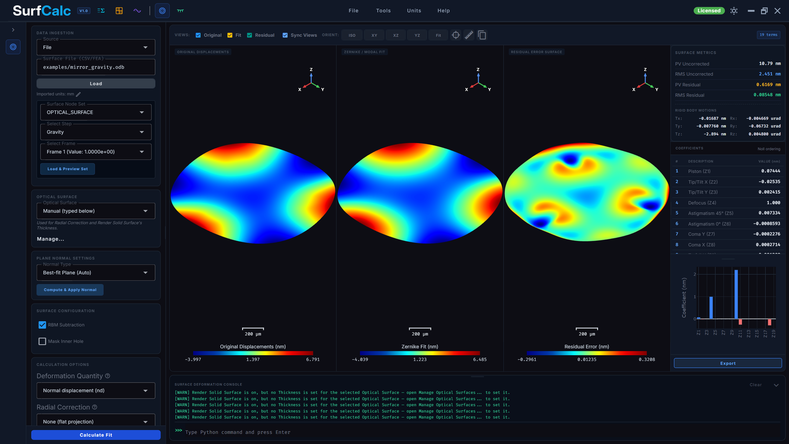
Step-by-Step Workflow:¶

1. Load FEA Model or CSV:

   • Click Browse Model to select a file. This launches the unified, unit-aware Import File Dialog, which contains embedded unit selectors directly inside the file picker. This allows you to configure import units (Coordinates & Displacements, Rotations, and Forces) in a single step during file selection, automatically propagating units across the workspace and Project Explorer.
   • Supported formats: Abaqus (.inp/.odb), Nastran (.bdf/.dat/.op2), Ansys (.mac/.dat/.rst), CSV coordinate lists, and the two optical grid formats below.
   • For FEA files, select the target Nodal Set, Step Name, and Frame Index to preview and import nodes. If the dropdown auto-selects a set whose name matches optical keywords (optical / opt / os / mirror), Calculate loads that set itself rather than warning that nothing is loaded yet. A fallback to Default (All nodes) still requires an explicit Load & Preview Set.
   • Optical grid formats: Zemax Grid Sag (.dat / .sag) and CODE V Grid Interferogram (.int) import directly — the same formats SurfCalc exports, so a surface can be round-tripped through an optical design tool, and a measured interferometer grid can be fitted or used as an Active Optics target. .dat is shared with Nastran and Ansys; SurfCalc tells them apart by inspecting the file's contents, so no manual choice is needed. A grid file is a sag map over a flat reference, so the sag becomes the surface's normal displacement with the base plane flat — there are no node sets, steps, or frames to choose.

   [!IMPORTANT] Optical Grid Import Caveats:

   CODE V .int files carry no spatial extent — the header records only the grid's row and column counts, never its physical size. Supply one of the two fields the Import dialog shows for this format: a Companion Grid Sag File, the .dat exported alongside it (exact, preferred), or a Grid Diameter, the clear-aperture width of the grid, assumed centred on the origin. Import stops with an error if neither is given.

   Zemax Grid Sag unused points are dropped. OpticStudio marks cells outside the aperture with a sag of 1×10¹⁰ or greater (or a non-finite sag). SurfCalc skips those cells on import, so a circular (or otherwise masked) grid comes in as that aperture rather than a filled square. SurfCalc's own Grid Sag export writes the same unused-point marker. A file that instead stores a real sag in every cell still imports as a rectangle; fitting that directly inflates circular-Zernike coefficients because the fit radius becomes the grid corner.

   [!IMPORTANT] Safe Read-Only FEA Access: To guarantee absolute safety of your finite element databases, all imported binary result files—including Abaqus (.odb), Ansys (.rst), and Nastran (.op2)—are accessed in strictly read-only mode (readOnly=True or binary read-only format). SurfCalc never modifies or writes to the original simulation databases.

   [!WARNING] Abaqus Installation Requirement: Extracting nodal displacement data directly from Abaqus Output Database (.odb) binary files relies on executing abaqus python under the hood to access the proprietary odbAccess library. This requires a local installation of Abaqus on the host machine; however, read-only results extraction from .odb files does not consume any Abaqus license tokens.

2. Configure Unit System:

   • Define input displacement and rotation units (e.g., m, mm, um, nm).
   • Select output display units. SurfCalc handles all conversion factors automatically.
3. Polynomial Fitting & Method Selection:
   • Deformation Quantity: Choose what the fit, Original/Fit/Residual panes, RMS/PV, Zernike coefficients, and Grid Sag / CODE V export all use:
     • Normal displacement (nd) — \(u\cdot\hat{n}\). Default. The optical surface error a ray sees, and the usual SurfCalc WFE quantity.
     • Local-Z sag (uz) — displacement along the aperture-frame Z. Matches what Zemax Grid Sag and CODE V SUR apply as extra height. Use this when the coefficients and the grid file must add in an optical design tool.
     • Changing the quantity marks the fit stale; re-run Calculate Fit. Active Optics keeps nd for the solve (its influence matrix is nd); its Zemax / CODE V export can still write local-Z sag.
   • Radial Correction: On a curved (powered) surface, a node that slides sideways is still moving along the nominal prescription — that in-plane motion alone changes its raw axial displacement even with zero real optical error. Left uncorrected, a fast/deep mirror can even report the wrong sign (e.g. a uniformly-heated parabola flattens, but its raw axial displacement reads as more curvature). Also available in Active Optics, Influence Matrix, and Load Case Combination — each module's own Radial Correction setting is independent (like RBM Subtraction), and each can reference a shared mirror from the Optical Surface Library.
     • None (default) — today's flat projection, unchanged. Correct for a near-flat surface; increasingly wrong as the surface gets faster/deeper.
     • Linear / Nonlinear — enter the surface's Vertex RoC and Conic Constant (k) (the fields appear once either is selected) or pick a saved Optical Surface, then re-run Calculate Fit. Nonlinear differs from linear only for large in-plane motion relative to the local radius of curvature; for most cases they agree closely.
     • With RBM Subtraction on, the rigid-body motion removed from a radially-corrected fit is a piston + 2-axis-tilt fit of the corrected scalar itself, not the ordinary 6-DOF vector fit — decenter and clocking don't change the axial sag/normal deviation of a rotationally symmetric surface, so this is the physically appropriate motion to remove once the geometric slide has already been taken out. The Tx/Ty/Tz/Rx/Ry/Rz readout still shows the raw 6-DOF vector fit for reference.
     • Validation status: verified against a published reference to 0.01% agreement on a thermal load; a gravity load currently agrees to 2.8–18% depending on term and is still under investigation. Default is None everywhere for this reason — treat a radially-corrected result as informative, not yet as fully validated as the uncorrected (flat-projection) fit.
   • Fit Method: Select the mathematical formulation that matches your mirror's aperture geometry:
     • Circular Zernike: Traditional circle Zernikes (Noll or Fringe indexing) orthogonal over a unit circle.
     • Annular Zernike (Mahajan): Orthonormal polynomials over an annular aperture (mirror with a central hole), using the obscuration ratio \(\epsilon\) derived from inner and outer diameters.
     • Rectangular Chebyshev: 2D tensor product Chebyshev polynomials sorted via Standard Triangular Sorting, ideal for rectangular/square mirrors.
     • Hexagonal Segment: Discrete Gram-Schmidt orthonormalized polynomials over regular hexagonal segments (with apothem and vertical flats), supporting auto-detected or manual flat-to-flat spacing constraints.
   • Zernike Indexing Type: For Zernike methods, choose between Standard (Noll) and Fringe indexing formats.
   • Terms Selection: Input the specific term range (e.g. 1-15) or comma-separated list of terms (e.g. 1,2,3,4,9,11) to include in the fit.
   • Normalization: Toggle the normalization checkbox to switch between normalized and unnormalized polynomial bases.
4. Mask Inner Hole (Central Obscuration), in the Surface Configuration section:
   • High-precision telescope mirrors frequently feature central holes. Toggle Mask Inner Hole to exclude that region.
   • Toggle Mask Inner Hole, then enter a known Hole Diameter (in the current input units shown on the field) or click Auto to detect it from the mesh. Enabling the checkbox alone does not detect a diameter.
   • SurfCalc keeps every surface node and only removes the fake Delaunay triangles that bridge the empty gap. With a diameter set, the toggle applies from import onward, not just at Calculate Fit, so nodal-area weighting, the Original pane, and the fit all agree.
5. Rigid Body Motion (RBM) Fit:
   • Toggle Remove RBM to isolate elastic surface deformation from rigid translation (\(T_x, T_y, T_z\)) and rotation (\(R_x, R_y, R_z\)).
6. Execution & Visualization:
   • Click Calculate (located at the bottom of the calculation options pane) to run the Weighted Least Squares (WLS) solver.
   • Visualizations automatically show the Original Surface, Zernike Fit Surface, and Residual Surface in the interactive 3D plotters.
   • Show Edges Default: Interactive 3D mesh lines default to Off for clean rendering.
7. Report Export:
   • Export detailed Optomechanical Summaries (_summary.txt), Zemax Zernike coefficient tables (_zemax_coefficients.txt), Zemax Grid Sag format files (_grid_sag.dat), or CODE V Grid Interferograms (_codev_interferogram.int) directly by triggering the Export Report option under the File menu. Grid Sag and CODE V files are Original, Fit, or Residual of the Deformation Quantity (nd or uz) — not the undeformed figure (Zemax/CODE V already have the nominal optic). Under Fields to export, tick any combination of Original, Fit, and Residual (default Residual, so the grid pairs with the Zernike coefficient file instead of double-counting low-order terms); each ticked field writes its own file. A progress bar in the toolbar shows which file is being written and lets you Stop between files. Coordinates default to millimetres; Imported or Displayed units are also offered.
   • Analysis Report (.html) — the shareable form of the same run, and the one to pick when the output is going to a person rather than another program. One self-contained file, branded with the SurfCalc logo, holding screenshots of all three viewports (Original / Fit / Residual, always captured face-on from the XY plane regardless of what angle you last orbited them to, and regardless of which panes are currently toggled visible), the fit setup, the uncorrected/residual RMS and PV figures, the six rigid-body components, the full coefficient table, and — if the surface came from a Load Case Combination — which cases were combined, with what multipliers, onto which reference mesh. It opens automatically in your default browser once written; use its Print to PDF to produce something you can attach to a design review. Nothing is linked externally — the logo and viewport images are embedded directly, not referenced — so the file still renders correctly after being emailed on its own. Capturing the report images resets nothing about your own view: each viewport's camera is restored right after its screenshot is taken, so you keep whatever angle you had before exporting.
     • SurfCalc deliberately ships no PDF engine; printing from the browser is the supported route to PDF, and the report carries print-specific styling so page breaks land between sections rather than through a table.
     • The .txt summary is unchanged and still written when ticked — keep it for grepping and diffing runs, and use the .html when a human has to read it.
   • Combined Surface (.csv) writes the displacement field back out in the same CSV format SurfCalc imports (X, Y, Z, UX, UY, UZ, NX, NY, NZ, Area, in metres) — the same format the Load Case Combination module produces.

Influence Matrix Generator Module¶

The Influence Matrix Generator decouples a multi-actuator FE model into individual single-actuator runs, generates solver decks and a batch runner, and compiles the completed solver results into the system matrix. The external FE solver is run outside SurfCalc.

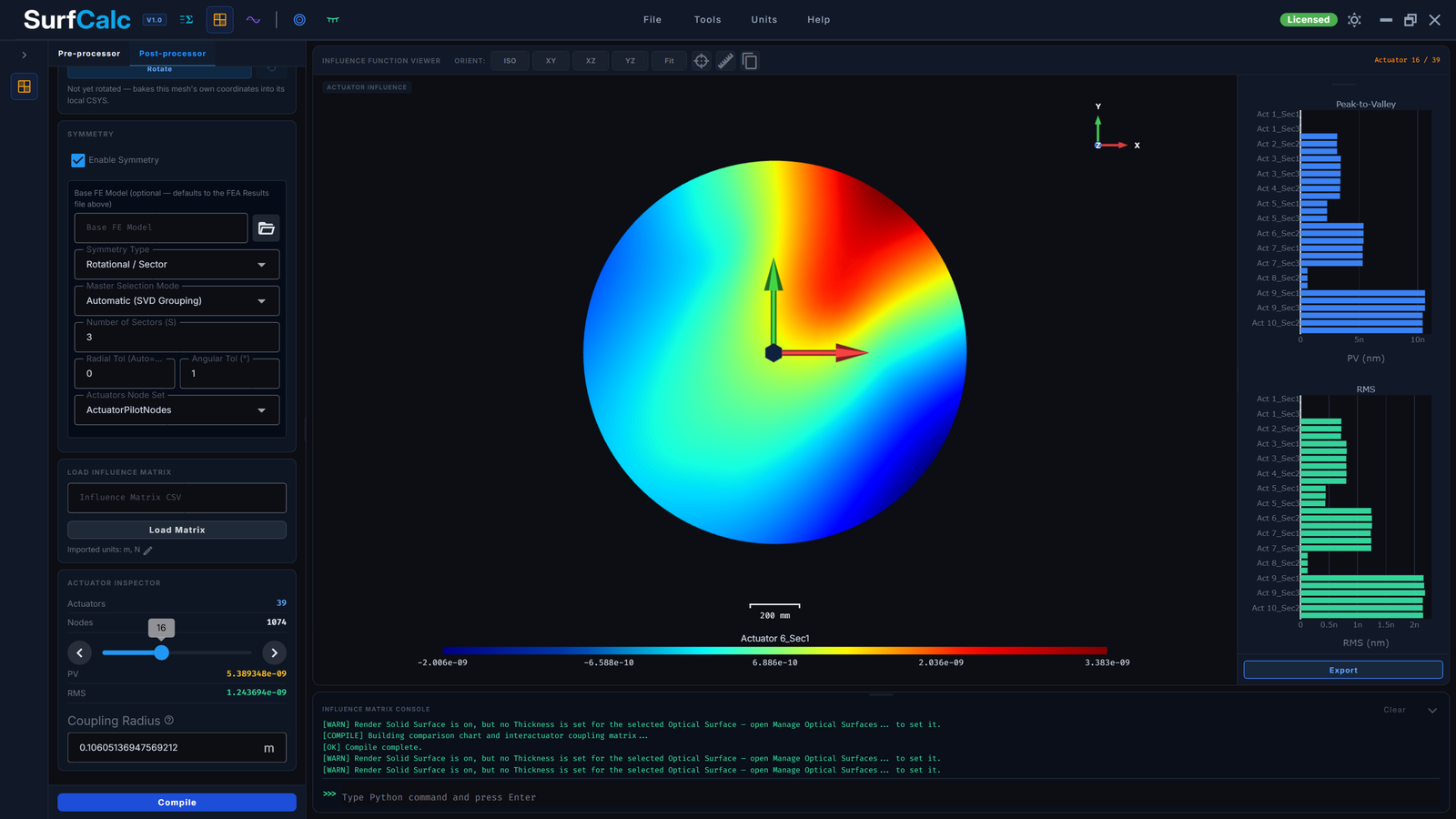
Step-by-Step Workflow:¶

1. Define Nodal Sets:
   • Optical Surface Set: The nodal set corresponding to the mirror's reflective surface.
   • Actuator Node Set: The specific nodes where actuator force/displacement loads are applied.

2. Configure Solver & Boundary Conditions:

   • Select the target FE solver: Abaqus, Nastran, or Ansys APDL.
   • Solver Executable Path: Displays standard execution commands (e.g. abaqus job=..., nastran ...). Customize the executable binary path as needed.
   • Template Load Selection: If the base model has existing loading/boundary condition cards defined for actuators, select a Template Load card from the dropdown to automatically perform actuator node and load configuration swapping.
   • Load Type & Value: Choose between Force and Displacement loads, and set the magnitude value (in consistent solver units).
   • Direction: Specify the load application axis (e.g., local surface normal or global axes).
   • Active Restraints: Degrees of freedom constraint applied to the active actuator node (e.g. unrestrained or locked).
   • Inactive Restraints: Boundary conditions applied to all other inactive actuators during a single actuator's run (e.g. locking UX, UY, UZ, ROTX to prevent rigid motion).

   [!WARNING] Commercial Solver Licensing Requirements: Running the generated finite element jobs requires a valid local installation and solver license (e.g., Abaqus, MSC Nastran, or Ansys APDL). SurfCalc writes a runner script, but does not launch or monitor the commercial solver itself.

3. Generate Solver Decks & Batch Runner:

   • Solving Strategy: Choose between Single Master Run (Fast) (solves all load steps inside a single deck/output database step layout for faster solving) and Sequential Runs (Low RAM) (writes individual deck files for each actuator node to run sequentially, which saves host memory).
   • Click Generate Solver Input File to generate the deck files (e.g., prefix_act_1.inp or prefix_master_influence.inp).
   • A specialized, single-solver Python batch runner script run_influence_matrix.py is written to the same directory.
4. Run Finite Element Analysis:
   • Close or save the project, then run the generated run_influence_matrix.py from a solver-configured terminal outside SurfCalc. Review the solver's own status/output files before compiling; SurfCalc does not provide an in-app Run FE Analysis command.
5. Post-Processing & Compilation:
   • Click Browse Results and select the folder containing the sibling results files (prefix_act_*.odb, prefix_act_*.op2, prefix_act_*.rst).
   • Select whether to project displacements onto the Local Surface Normal or along global coordinate axes.
     • Radial Correction: a compile-time setting, next to Remove Rigid Body Motion — see Radial Correction above. Since Influence Matrix has no per-actuator local aperture frame the way Surface Deformation does, the correction uses each actuator's own mesh recentred at its own area-weighted centroid as the assumed aperture centre. Nonlinear is only available when the results file's coordinate and displacement units match (declared in Data Ingestion); otherwise it is blocked with a specific message. The setting is baked into the compiled matrix and recorded in the exported CSV/summary — recompile to change it, editing the dropdown afterward does not retroactively recorrect an already-compiled matrix.
     • Symmetry & Expansion Options: To expand a simulated master subset of actuators to a full-symmetry matrix, expand the "Symmetry & Expansion Options" collapsible box:
       • Check Enable Symmetry Expansion.
       • Choose Symmetry Type: Rotational (for S sectors) or Bilateral (for reflection across a custom plane).
       • Configure parameters: Number of Sectors (e.g. 6 or 12) or Plane Angle in degrees.
       • Master Selection Mode: Choose between Automatic (SVD Grouping) (which automatically determines sector bounds and actuator groups using SVD) and Manual Sector Bounds (which restricts master selection strictly within a user-defined Min/Max angle range).
       • Custom Tolerances: Adjust the Radial Tolerance (automatically scaled to your active coordinate unit mm/um/nm) and Angular Tolerance to customize the actuator proximity matching threshold. Set Radial Tolerance to Auto or 0.0 to use the robust automatic minimum.
       • Verify & Preview: Click Preview Preprocessing Symmetry or Verify & Show Symmetry Mapping to visualize the sectors, master actuators (highlighted in magenta), and "virtual" symmetric actuators (highlighted in yellow/orange) in the interactive 3D plotter.
       • Asymmetry Alerts: SurfCalc automatically scans boundary support constraints (BCs) and warns you in the console if asymmetric support restraints are detected, helping you avoid physically inaccurate influence matrices.
       • SurfCalc will automatically handle back-rotation, bilateral reflection, and continuous linear/nearest interpolation to cleanly expand the columns.
   • Performance Caching Optimization: Under the hood, spatial lookup mappings are automatically cached across the extraction loop. If the mesh structure remains static across different actuator runs, SurfCalc bypasses the expensive \(O(M \cdot N \log N)\) KDTree reconstruction on every loop iteration, providing an instant \(M\times\) speedup.
   • Click Extract & Export Matrix (anchored at the bottom of the Results pane) to load all displacements, project them, assemble them into the columns of the influence matrix, and export the .csv matrix file.
   • A human-readable _summary.txt is written alongside the matrix CSV, recording the source results file, units, node and actuator counts, the resolved local CSYS, the per-actuator PV/RMS magnitudes, and — most importantly — the symmetry settings that were actually applied, so a reviewer can tell which actuators were solved directly and which were synthesized by expansion.

Active Optics Correction Module¶

The Active Optics workspace uses the compiled influence matrix to compute the optimal forces/displacements required to minimize surface RMS error.

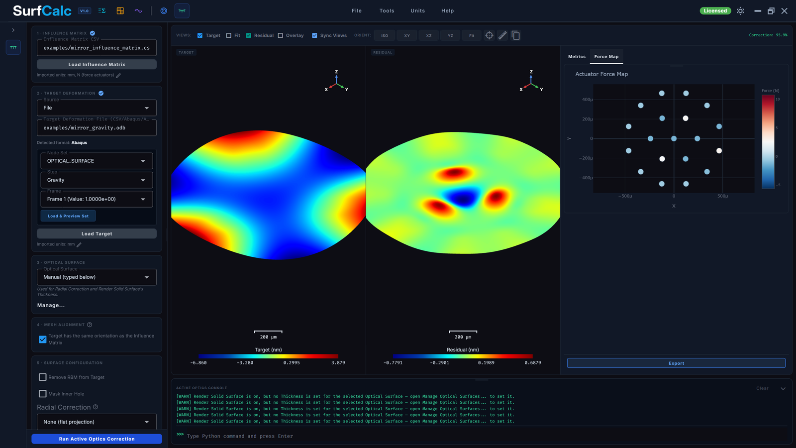
Step-by-Step Workflow:¶

1. Load Deflection and Influence Matrix:
   • Target Deflection Source: Choose between Current Surface (Tab 1), External CSV File, or Model File (imports displacements directly from Abaqus .odb, Nastran .op2, or Ansys .rst database files).
   • Zemax Grid Sag (.dat / .sag) and CODE V Grid Interferogram (.int) files can also be loaded as the target, letting a measured or optically-designed surface drive the correction directly. The sag is already a normal departure by definition of the format, so it is used as the target deformation as-is. The same caveats as the Surface Deformation module apply: an .int needs a companion .dat or a stated grid diameter to place it in space, and unused Grid Sag cells (sag ≥ 1e10) are dropped so the target is the clear aperture, not a filled square.
   • Import the system Influence Matrix CSV.
2. Apply Limits/Constraints:
   • Toggle Enable Actuator Limits and specify upper and lower bounds (e.g. maximum tensile or compressive forces).
   • Check Remove RBM from target to subtract rigid body translations/rotations from the target profile prior to calculating active optics commands.
   • Radial Correction (Surface Configuration section) — see Radial Correction. Only the target is corrected; the influence matrix is already a scalar (each Actuator_N column is a pre-projected value with no displacement vector), so there is nothing to correct on that side. A Grid Sag / CODE V interferogram target, or a target CSV carrying only a legacy scalar column (no UX/UY/UZ), has no vector to correct and shows a note explaining why instead of the Vertex RoC / Conic fields.
     • If the loaded influence matrix was compiled with a different Radial Correction setting than the target (or was compiled without correction while the target is corrected, or vice versa), a warning appears explaining the mismatch — it never blocks the solve, since comparing a corrected and uncorrected result is itself a valid way to check the correction's effect, and a hand-made or third-party influence matrix will never carry the provenance needed to check it at all.
3. Run Correction:
   • Click Compute Active Fit at the bottom of the parameters panel. If the target is an FEA file whose dropdown auto-selected a keyword-matched optical node set that has not been previewed yet, the correction loads that set first (same auto-load as Surface Deformation's Calculate). Default (All nodes) still requires an explicit Load & Preview Set.
   • SurfCalc executes a bounded linear least-squares solver (Trust Region Reflective algorithm) if limits are enabled, or a standard unconstrained WLS solver.
   • The display outputs:
     • Original RMS Error and Corrected RMS Error.
     • Active Correction Factor (the percentage reduction in surface RMS).
     • Interactive 3D views of original vs. corrected shapes.
4. Actuator Command Output:
   • View the detailed command list table, which lists each actuator, its node ID, the calculated command value, and its status (e.g. OK or Saturated).
   • Click Export Actuator Commands to write force commands to a CSV file.
   • The same Export Report dialog writes Zemax Grid Sag / CODE V files of Original, Fit, and/or Residual. Grid Quantity defaults to Local-Z sag (uz) — \(u_z = u_d n_z\), the extra height those formats apply — so a residual can go straight into OpticStudio or CODE V. The solve itself stays nd. Pick Normal displacement (nd) to write the solver scalar as-is. Residual CSV is always nd (re-importable as an AO target).
   • The same dialog also offers an Analysis Report (.html) — one self-contained, SurfCalc-branded file with screenshots of all four viewports (Target/Fit/Residual/Overlay, always face-on from the XY plane), correction quality (RMS/PV before and after, RMS Reduction, AFI), solve setup, Monte Carlo tolerance results if you ran them, and the full actuator table. It opens automatically in your browser; print to PDF from there to share it. Same file format and light/dark toggle as Surface Deformation's report.
5. Reliability & Diagnostics Dashboard:
   • To prevent structural failure (such as glass face-sheet cracking) from localized opposing forces, utilize the Reliability & Diagnostics dashboard under the correction options:
     • Solver Regularization: Choose between Standard (Least Squares), Tikhonov Regularization (Ridge Regression to penalize absolute forces), or Laplacian Regularization (Smoothing to directly penalize actuator fighting and localized shear).
     • Regularization Parameter (\(\alpha\)): Specify manually or click Auto-Detect \(\alpha\). SurfCalc sweeps candidate parameters to automatically identify the knee of the L-curve.
     • Monte Carlo Simulation: Model physical actuator tolerances. Specify Sensor Noise (nm), Actuator Gain Error (%), Actuator Offset Noise (N), and the number of Trials (e.g., 1000). Click Run Monte Carlo to execute.
     • Interactive Diagnostic Plots: Review the diagnostics tabs:
       • 2D Force Map: View the concentric circles of the actuator layout, colored dynamically by force direction and magnitude to visually identify stress concentrations.
       • L-Curve: Examine the log-log plot to verify the optimal parameter knee.
       • Monte Carlo Yield: Analyze the probability density histogram of corrected surface RMS errors, highlighting the 95th and 99th percentile yield thresholds.

Load Case Combination Module¶

A STOP analysis normally produces separate FEA runs for gravity, thermal soak, and wind. The Load Case Combination module combines them into one deformation field, which can then feed one or more Surface Deformation fits (with different fit bases) and/or an Active Optics target — one combination, several downstream analyses.

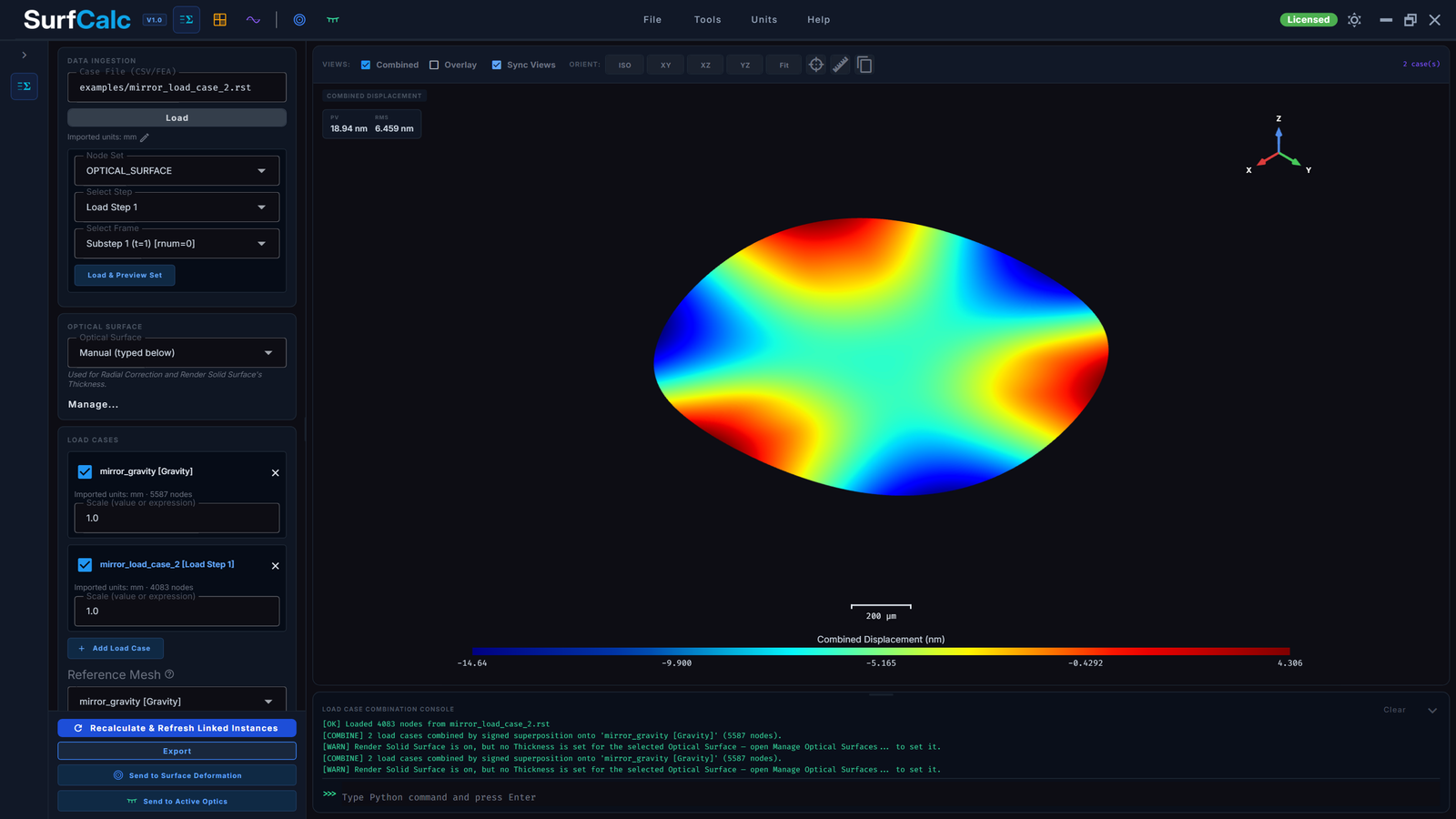
Step-by-Step Workflow:¶

1. Add Load Cases:
   • Click Add Load Case to lay out an empty slot before its model exists, or Load in Data Ingestion to import the first case directly. Each case is loaded through the same unit-aware Import dialog as Surface Deformation, so cases saved in different units combine correctly.
   • Each case shows its imported units and node count beneath its name — a deliberate double-check, since cases are converted to a common basis before combining and a case imported under the wrong unit would otherwise be invisible in the result.
   • Give each case a signed Multiplier (e.g. 1.0 gravity, 0.6 thermal, -1.0 to reverse a case's sense), or untick a case to exclude it without removing it.
   • Click a case's name to load its import settings back into Data Ingestion — the source file, units, and (for FEA) node set, step and frame it was built from. From there you can inspect it, change any setting, or browse to a different file, then click Load (or Load & Preview Set) to replace that case's model in place. Its multiplier and enabled state are preserved, since those are decisions about the case rather than properties of the file.
   • Right-click a case → Duplicate copies it into a new slot right below — same file, units, multiplier and alignment, plus its already-loaded mesh (the same menu also offers Remove). This is the quick way to run the same model under a different load step or frame: duplicate, pick another Step/Frame in Data Ingestion (the copy is already selected), click Load & Preview Set, then tick the copy's checkbox to include it. The copy is added unticked on purpose — until its own model is loaded it holds exactly the same field as its source, and combining both would double the result.
2. Reference Mesh & Alignment:
   • Cases need not share a mesh. The most refined mesh becomes the reference by default (or pick one explicitly under Reference Mesh), and every other case is recentred on its own area-weighted centroid and interpolated onto it. Identical meshes skip interpolation entirely.
   • Mesh Alignment (shown for the selected case once more than one case is active) — cases need not share an orientation either. Leave Same orientation as reference case ticked for the common situation where every case came out of the same model. Untick it to declare that case's local CSYS as three points in its own coordinates (Origin, X-Axis Point, XY-Plane Point), typed directly or read from the file's own positioning-CSYS cards, then click Apply Alignment. The case is then rigidly registered onto the reference case's frame — coordinates, displacement vectors and surface normals all rotate together.
   • This is the same 3-point convention Active Optics uses to register a target onto an influence matrix, and it behaves the same way when no frame is declared: the combination stays centroid-aligned only rather than inferring a rotation from a best-fit plane or principal axes. That restraint is deliberate — the in-plane axes of a rotationally symmetric mirror are arbitrary, so a guess would silently rotate a case instead of admitting it could not align it.

3. Combination Mode:

   • Signed Superposition — a scaled vector sum. Use for correlated contributors whose relative sign is meaningful. The result is a physically realizable deformation state.
   • RSS Envelope — combines the scaled normal displacements in quadrature. Use for uncorrelated contributors (thermal noise, wind buffeting). The result is a statistical bound, not a realizable deformation state: its Zernike coefficients bound the error budget but do not describe a physical surface shape.
   • The combined result updates live as cases, multipliers, alignment, or combination mode change — there is no separate "Calculate" step. If an FEA case's dropdown auto-selected a keyword-matched optical node set that has not been previewed yet, the Engineering Console's calculate() and Grid Sweep load those matched pending cases first (the same auto-load as Surface Deformation). Default (All nodes) still requires an explicit Load & Preview Set.
   • Surface Configuration on the combined result mirrors Surface Deformation: RBM Subtraction, Mask Inner Hole (manual diameter or Auto detect), and Radial Correction (see Radial Correction) — this governs the combined-result viewport and its Peak RMS/P-V readout.
   • This module's own Radial Correction setting is what a Grid Sweep's Combined Surface and Surface Deformation Fit evaluate stages see (the latter via the linked instance's own Radial Correction, forwarded automatically). The Active Optics Correction evaluate stage is the one exception: it consumes the combined field's already-computed normal displacement, so it always reflects this module's Radial Correction setting, never the linked Active Optics instance's own — a warning appears in the console if the two differ, since that setting has no effect on the sweep.

   [!NOTE] Load Case Combination (and every other import/calculate path) requires an active license or trial. Without one, combine and sweep stay blocked.

   Grid Sweep¶

   Load magnitude and combination are the genuine unknowns in a STOP analysis — how hard is gravity really pulling at this zenith angle, how much does the thermal soak actually vary — so this is where a parametric study belongs, not in a fit method's own settings.

   • Independent Variables: click Add Variable to name a scalar (e.g. g, theta), then reference it in any case's Multiplier field as an expression (g, cos(theta), 2*g). Two cases can share one variable to model something like a rotating gravity vector.
   • Grid Sweep: tick a variable to sweep it and set its Min / Max / Step — the combination re-runs once per grid point across the Cartesian product of every ticked variable's range.
   • Evaluate Through decides what a grid point is judged by. Every metric the chosen stage computes is its own sortable column in the results table — click a header to rank by it. The scatter chart's X axis is a swept variable; its Y axis is whichever metric column you pick.
     • Combined Surface — the raw combined field's own Peak RMS and Peak P-V (the original behaviour).
     • Surface Deformation Fit — pick a linked Surface Deformation instance; each grid point runs through that instance's own fit settings (fit method, term selection, RBM subtraction, everything already configured there). Columns: Residual RMS/P-V and Fit RMS/P-V. Answers "which load combination leaves the worst uncorrectable error?" Click a row to load that grid point and see its Fit and Residual surfaces next to Combined.
     • Active Optics Correction — pick a linked Active Optics instance; each grid point registers onto that instance's own influence matrix and solves with its configured actuator limits and regularization. Columns: Residual RMS/P-V, Correction Factor, Actuator Fighting Index, Max Actuator Command, and Over Budget (Yes/No — click that header to bring every over-budget case to the top). Rows tinted amber mark a grid point where at least one actuator saturated at its configured limit. Click a row to see the corrected Fit and Residual on the influence-matrix mesh.
     • Either linked instance's own settings decide how a point is evaluated; Load Cases only decides what varies. Nothing is configured twice.
   • After a sweep finishes, the worst Residual RMS point is loaded automatically (Peak RMS when evaluating Combined Surface, Residual RMS for a Surface Deformation fit or Active Optics correction) so Combined / Fit / Residual show that case. Click a column header to sort by it, or a row to load a different grid point.

4. Export or Hand Off the Result:

   • Export (sidebar footer, or the Sweep Results panel after a run) opens the same options dialog Surface Deformation and Active Optics use. Tick Sweep Summary (.csv) for every grid point's columns, and/or Current Combined Surface (.csv) for the loaded point's combined field (X, Y, Z, UX, UY, UZ, NX, NY, NZ, Area, in metres — re-importable in any module). When Evaluate Through is a Surface Deformation fit or Active Optics correction, the dialog also offers that stage's own exports for the currently loaded grid point — Analysis Report (.html), Summary (.txt) and Zemax coefficients for a fit, actuator forces/displacements for a correction, plus Zemax Grid Sag, CODE V interferogram, and Residual Surface CSV.
   • Send to Surface Deformation creates a new Surface Deformation instance fed by the combined field and keeps it linked — recombining later (a new multiplier, an added case) refreshes every linked instance automatically. Click it again to feed a second Surface Deformation instance with a different fit basis from the same combination.
   • Send to Active Optics creates a new Active Optics instance whose target is the combined field, kept linked the same way.
   • If a linked producer instance is later deleted, its consumers keep their last-loaded data but stop refreshing — they are not deleted themselves.

Thermal Free-Growth Case Type¶

Most cases feed Load Case Combination from an already-solved FEA displacement field. Thermal Free-Growth is the one exception: it takes a nodal temperature field instead — a standard by-product of a thermal FEA run, or a hand-built CSV for an early trade study — and computes a displacement field from it directly, without needing a coupled thermal-structural solve at all.

[!WARNING] This computes the field as if every node grows independently and radially outward from a reference point, in proportion to its own local temperature change: u = CTE × ΔT × (P − P_ref). That is the exact thermoelastic solution only for a spatially uniform ΔT (a rigid similarity expansion). For a non-uniform field it is a standard engineering approximation: it assumes a kinematically isostatic mount (no mount reaction) and ignores the internal stress a real elastic body develops resisting differential expansion between neighboring nodes at different temperatures (no CTE-mismatch/bond-line stress, no print-through). This is the same limitation Sigmadyne's SigFit documents for its own free-growth handling — this feature reaches parity with that, not beyond it. Use it for an early trade study before a thermal-structural FEA run exists, not as a substitute for one once it does — a real coupled solve (imported like any other FEA case) is always more accurate.

• Set Case Type to Thermal Free-Growth on the case (next to its Multiplier). This replaces the case's Data Ingestion panel with a Thermal Free-Growth panel and hides the FEA node-set/step/frame controls, which don't apply.
• Load the temperature field: Browse to a CSV with X, Y, Z (already in SI metres — there is no unit-conversion dialog for this file type in this release) and a T or TEMP column, plus an optional AREA column used only to weight the default reference point below.
• Reference Temperature — the stress-free/mounting temperature, in the same units as the file's T/TEMP column. There is no default: leaving it blank and computing anyway would silently assume a value, which is exactly the kind of wrong-number-with-no-warning this codebase's other guards (Radial Correction's best-fit-plane check, its conic-domain-overrun check) exist to prevent.
• CTE — pick an Optical Surface from the library to use its stored CTE (see Optical Surface Library above), or type a manual CTE (/K) value. The library value takes precedence when both are set.
• Reference Point — Centroid (the field's own area-weighted centroid, the default) or Custom to type an explicit (X, Y, Z) — e.g. a real mount point, when the geometric centroid isn't the right growth origin.
• Click Compute Free Growth to populate the case's displacement field. It then combines with every other case exactly like an FEA-sourced one — Multiplier, RSS/Superposition mode, and downstream Surface Deformation/Active Optics handoff all work unchanged.

Bending Modes Module¶

Rather than fitting an idealized analytical basis (Zernike, Chebyshev, hexagonal), the Bending Modes module extracts a basis directly from an FEA modal (eigenvalue) analysis — or a hand-built CSV of mode shapes — so a downstream Surface Deformation fit can use the mirror's actual structural bending shapes instead of an assumed optical polynomial family.

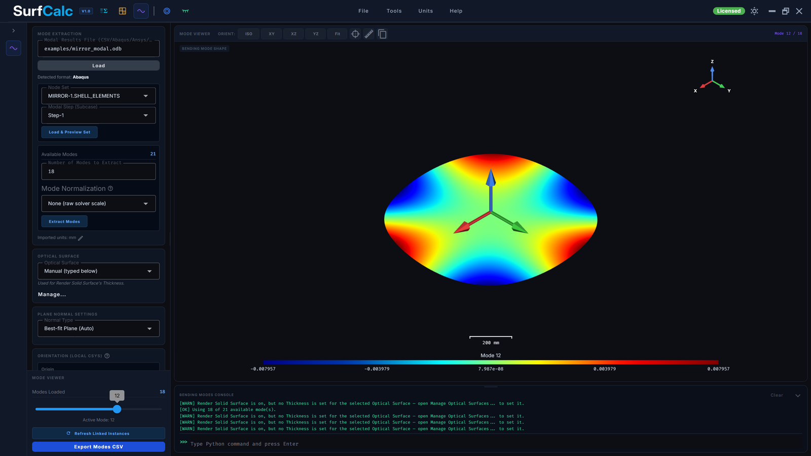
Step-by-Step Workflow:¶

1. Load a Modal Results File:
   • Click Browse (or drag-and-drop onto the viewport) to select a Modal Results File — a CSV of Mode_1, Mode_2, ... columns, or an Abaqus/Ansys/Nastran modal-analysis database. The format is auto-detected and shown under Detected format.
   • For FEA files, select the Node Set and Modal Step (Subcase), then click Load & Preview Set to read the available modes. If the dropdown auto-selects a keyword-matched optical set, Extract Modes loads that set itself rather than warning that nothing is previewed yet. Default (All nodes) still requires an explicit Load & Preview Set.
2. Extract Modes:
   • Set the Number of Modes to Extract (up to the reported Available Modes count).
   • Choose a Mode Normalization: None (raw FEA eigenvector scale), Peak (each mode scaled so its peak magnitude is 1), or RMS (each mode scaled so its own area-weighted RMS is 1) — Peak/RMS make a later fit coefficient read as a direct physical amplitude rather than an arbitrary solver scale.
   • Click Extract Modes.
3. Optical Surface & Plane Normal / Orientation:
   • Optical Surface picks a mirror from the Optical Surface Library (see below) — Bending Modes has no Radial Correction concept, so this is only consumed by Render Solid Surface's Thickness in the viewport right-click menu.
   • Normal Type controls how the surface normal used to project FEA displacements is determined: compute from a best-fit plane, or supply a Custom Vector.
   • Orientation (Local CSYS) lets you declare the mesh's local frame (Origin, X-Axis Point, XY-Plane Point) the same way Surface Deformation and Load Case Combination do, so a mode basis registers consistently with the surfaces it will be fit against.
4. Review in the Mode Viewer:
   • The Mode Viewer footer control (fixed at the bottom of the sidebar) scrubs through Active Mode via a slider, showing each extracted mode shape one at a time in the 3D viewport.
   • Deformation Scale (Auto / Custom / Auto-Equalize) is controlled from the shared 3D viewport right-click context menu, the same as Surface Deformation, Influence Matrix, and Active Optics — there is no separate scale control in the sidebar.
   • Export Modes CSV writes the current mode basis out in the same Mode_N column format SurfCalc imports, so it can be archived or reused without re-extracting.
5. Link to Surface Deformation:
   • In a Surface Deformation instance, set Fit Method to Bending Modes, then set Modes Source to Bending Modes Instance and pick the source instance from the dropdown, then click Link.
   • The linked fit refreshes automatically whenever the source Bending Modes instance re-extracts, re-normalizes, or reorients — click Refresh Linked Instances on the Bending Modes side if a linked fit ever looks stale (e.g. right after reopening a project). Click Unlink on the Surface Deformation side to switch back to a plain CSV modes path.

Sensitivity Matrix Module¶

Computes a first-order (paraxial) rigid-body tilt/decenter → line-of-sight sensitivity matrix from an optical prescription — an ordered sequence of mirrors and/or lenses with known axial position and power. This replaces guesswork or a hand-authored sensitivity CSV with a real optics calculation, and feeds Image Motion directly.

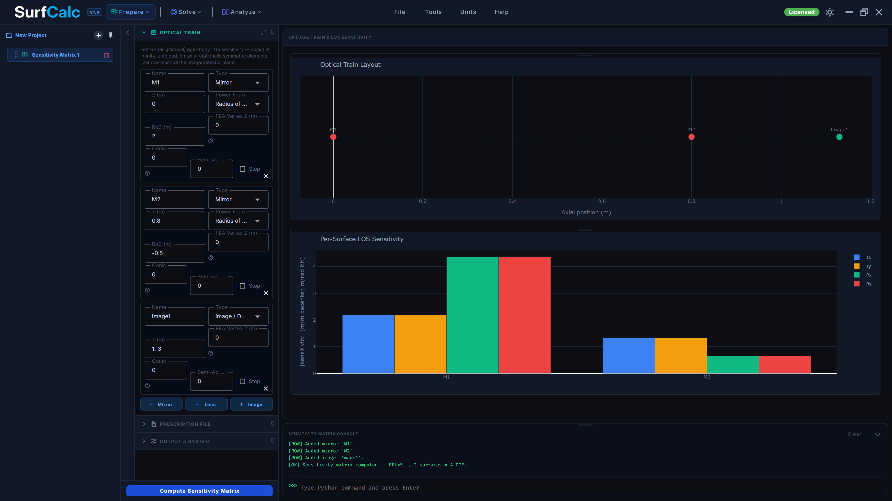
This is first-order/paraxial only: no aberration sensitivity, no despace (Tz) or clocking (Rz) sensitivity (both are exactly zero at this order for a rotationally symmetric surface), object at infinity, and an unfolded on-axis train.

Step-by-Step Workflow:¶

1. Build the Optical Train:
   • Click Mirror, Lens, or Image in the sidebar to add a row. The train must end with exactly one Image row (the detector/focal plane); every other row's Z (m) (axial position) must strictly increase along the train.
   • For each mirror or lens, set Power From to Radius of Curvature, Focal Length, or Optical Surface Library (pulling the radius of curvature from a mirror already defined in the shared Optical Surface Library, resolved at compute time).
   • Set FEA Vertex Z (m) for each element — its own vertex position along that element's own deformation file's global Z axis, used later by Image Motion to correctly reduce a fitted rigid-body motion to that element's decenter. Leave at 0.0 only when the FEA mesh's own origin already sits at the vertex.
   • Import from Zemax/CODE V: rather than typing each row by hand, click the folder icon under Prescription File and browse to a real Zemax OpticStudio (.zmx) or CODE V (.seq/.len) optical prescription — the format is auto-detected, the same one dialog also accepts a SurfCalc prescription CSV. Each surface becomes a row (mirror, lens, or the image plane), with its radius, thickness, conic, and semi-aperture carried over; the source file's own SURF n/S n label is kept as Source Surface for traceability. Three things are handled explicitly rather than silently:
     • Unfolded automatically. A real prescription writes a negative thickness after every mirror reflection; the importer un-negates these so the resulting Z (m) values are the physical (unfolded) path length this engine's on-axis model requires. A console [WARN] line reports how many segments were unfolded.
     • Object must be at infinity. SurfCalc's paraxial engine has no finite-conjugate mode — a prescription with a finite object distance is refused outright, naming the distance found.
     • A refractive (lens) element is imported but flagged "Needs Review." Its focal length can't be derived from radius/thickness alone without a glass catalog, which this importer doesn't have — the row comes in with Focal (m) = 0.0 and a note naming the glass; enter the element's known EFL before computing. Compute Sensitivity Matrix stays disabled while any row needs review. Off-axis, tilted, or non-sequential (zoom/NSC) prescriptions are refused entirely rather than imported wrong — SurfCalc's model is on-axis and sequential only.
     • Conic and Semi-Ap (m) on each row are metadata only, kept for round-trip fidelity and display — the sensitivity calculation itself uses only the vertex radius, per this module's first-order scope (see below).
     • Radius-of-curvature sign is carried over from the source file exactly as written, on the understanding that both vendors' convention already matches SurfCalc's own (positive = concave/converging) — but this has not been cross-checked against a real vendor-exported file (see docs/VALIDATION.md §7), so sanity-check the computed EFL/BFD against the source file's own reported value after import.
2. Choose an Output Mode: Image Plane (metres of image motion per metre of decenter, per radian of tilt) or Sky Angle (radians of sky angle per unit input — only valid for a train with a finite effective focal length).
3. Compute Sensitivity Matrix: reports the train's Effective Focal Length, Back Focal Distance, and how far the entered image plane sits from the true paraxial focus (not an error — a real detector is often placed off the ideal focus deliberately; sensitivities are computed at the image plane as entered).
4. Export or Send to Image Motion:
   • Save Prescription CSV / the folder-browse button next to Prescription File round-trip the optical train itself.
   • Save Sensitivity Matrix CSV writes the computed matrix in the format Image Motion consumes directly.
   • Export HTML Report writes a self-contained analysis report (the Optical Train Layout and LOS Sensitivity charts — still pan/zoom/hover-able in the exported file — system metrics, the resolved prescription, and the full sensitivity matrix) via the same shareable HTML format Surface Deformation and Active Optics produce — opens in your browser; print to PDF from there to share it.
   • Send to Image Motion creates a new Image Motion instance already linked to this one — the linked instance's sensitivity matrix refreshes automatically every time this Sensitivity Matrix instance recomputes.

Image Motion Module¶

Combines each optical surface's real deformation with a sensitivity matrix into a line-of-sight (LOS) error budget — the dominant image-quality driver for many imaging payloads, especially reaction-wheel/microvibration-induced jitter.

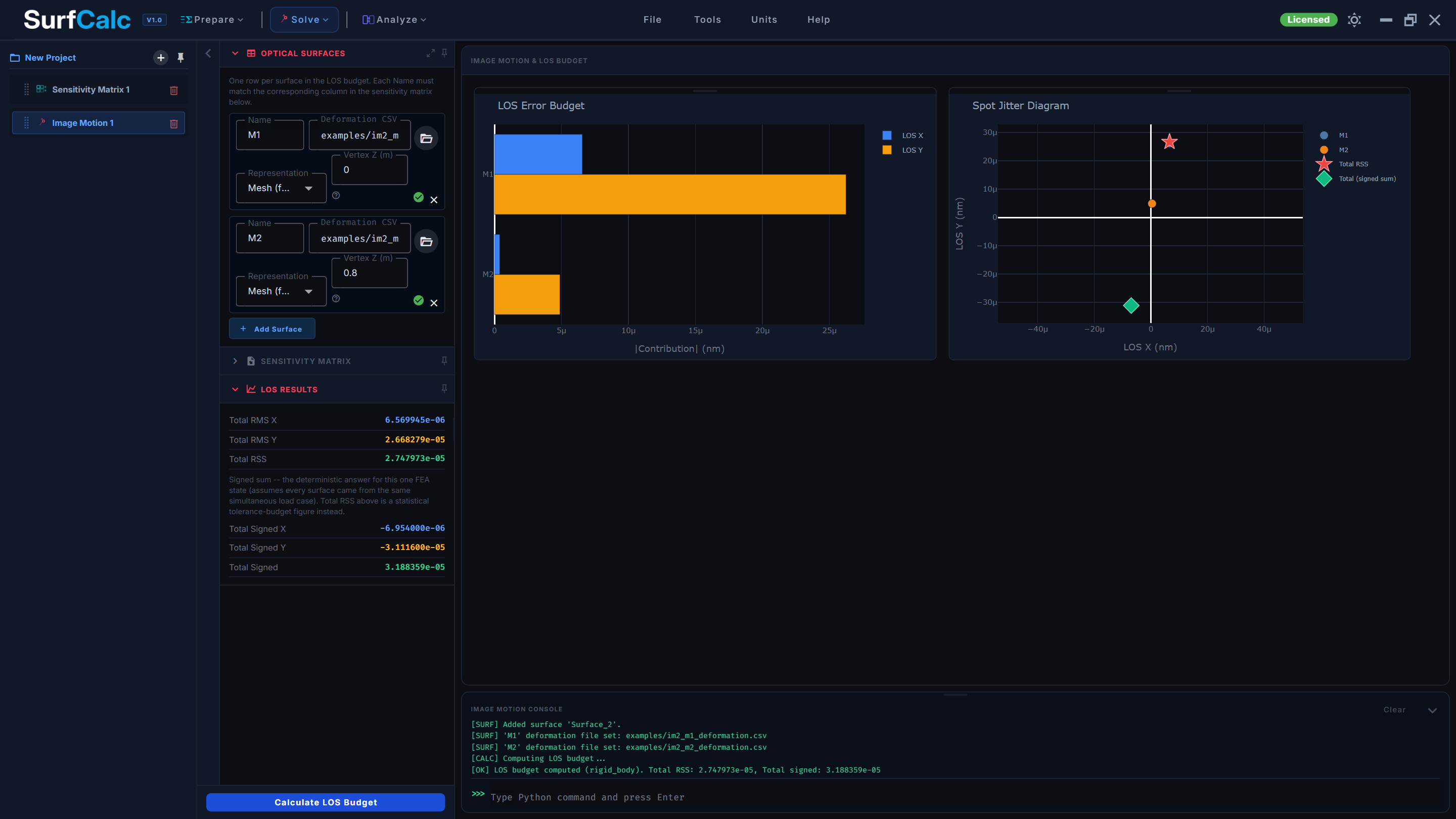
Step-by-Step Workflow:¶

1. Define Optical Surfaces:
   • Click Add Surface for each surface in the LOS budget. Each row's Name must match the corresponding element name in the sensitivity matrix.
   • Click the folder icon to browse to that surface's deformation data (a CSV of X, Y, Z, UX, UY, UZ, and optionally AREA, in SI units).
   • Set FEA Vertex Z (m) for each surface — see the Sensitivity Matrix workflow above; this must match the corresponding prescription row's own value for the reduction to be correct.
2. Load a Sensitivity Matrix: browse to a CSV directly, or — the recommended path — click Send to Image Motion from a Sensitivity Matrix instance, which creates and links a new instance automatically. The panel shows which format was detected:
   • Rigid-Body (Tx/Ty/Rx/Ry) — a real Sensitivity Matrix module export (2 rows x 4 columns per mirror).
   • External 6-DOF (Tx/Ty/Tz/Rx/Ry/Rz) — a 6-row, one-column-per-mirror matrix as typically exported by a full ray-traced optical model's own perturbation analysis (Zemax/CODE V), rather than this app's first-order engine. Unlike the Rigid-Body path, piston (Tz) and clocking (Rz) are read too, since a real model — unlike this app's on-axis paraxial one — can have genuine sensitivity to both. This format has only one output axis (there is no separate X/Y split), so its results show up under Total Signed only, with the RSS/signed Y figures reading zero.
   • Legacy (UX/UY RMS) — a hand-authored CSV predating the Sensitivity Matrix module, kept for backward compatibility but blind to a pure rigid-body tilt, which is exactly why one of the two paths above is recommended instead.
3. Calculate LOS Budget: reports two totals that answer different questions — Total RSS (the root-sum-square across surfaces, a statistical tolerance-budget figure) and, when a Rigid-Body or External 6-DOF matrix is loaded, Total Signed (the algebraic sum, the deterministic answer for this one FEA state — valid when every surface's deformation comes from the same simultaneous load case). The LOS Error Budget and Spot Jitter Diagram plots both update; the jitter diagram marks the RSS total with a star and, in Rigid-Body mode only (the format with an actual X/Y split), the signed total with a diamond.

Random Response Budget Module¶

Turns an FEA random-vibration result into the same kind of RMS/PV/Zernike-coefficient report SurfCalc already produces for a deterministic deformation — see docs/THEORY_MANUAL.md §17 for the math. This is not a random-vibration solver: SurfCalc never computes a mode's random-response amplitude itself. You run the random-vibration solve in your own FEA tool and request one extra output: each mode's own modal-coordinate 1-sigma RMS response (σ_k), the same physical scale as the mode shape it belongs to. This is usually not default solver output and needs an explicit request — see the per-solver notes below.

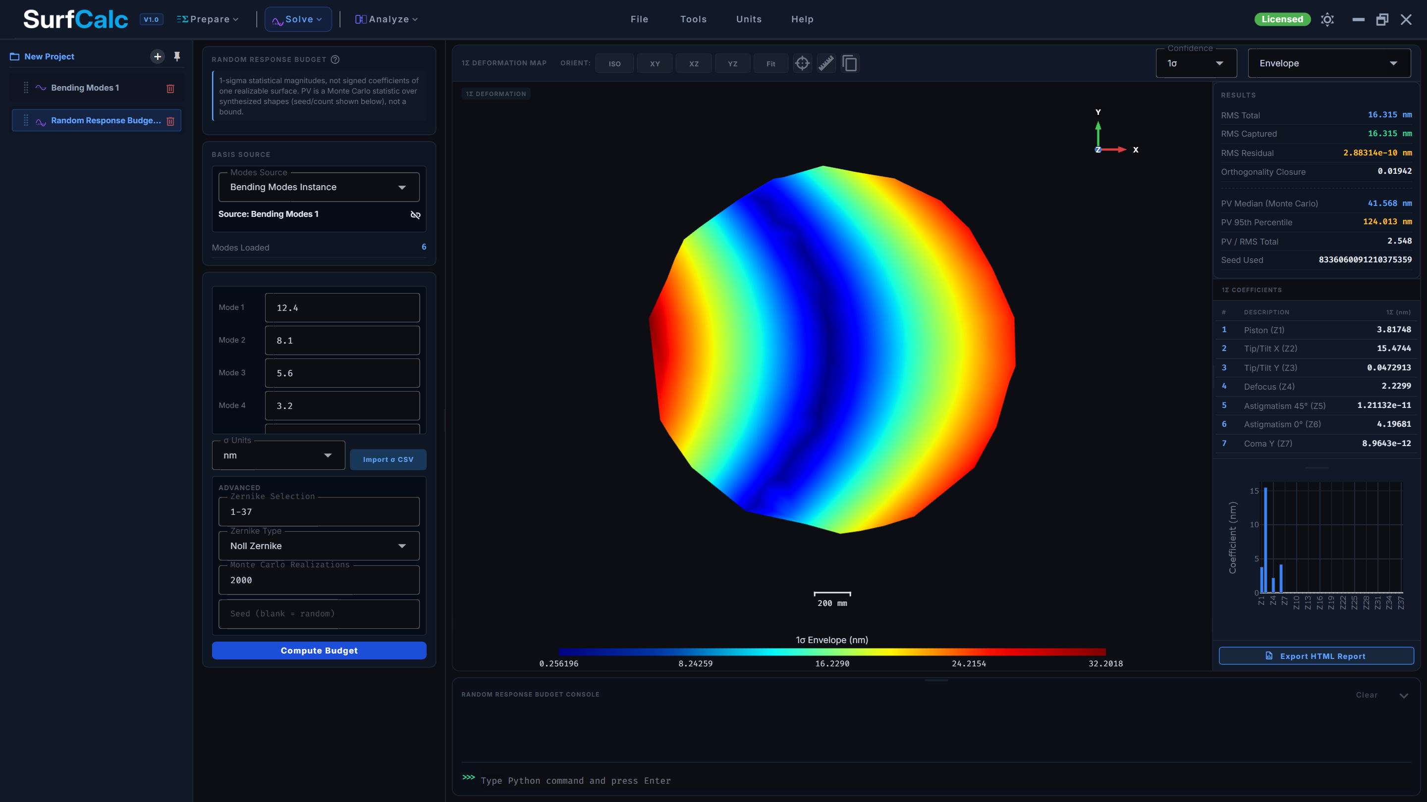
Step-by-Step Workflow:¶

1. Choose a Basis Source:
   • Bending Modes Instance (recommended) — pick an existing Bending Modes instance from the dropdown and click Link. The basis refreshes automatically whenever the source instance re-extracts, re-normalizes, or reorients; the per-mode σ table is cleared and a banner shown whenever that happens, since a σ_k is only meaningful against the exact mode shapes and basis it was entered against. Click the unlink icon next to Source: to switch back to a plain CSV path (the last-loaded basis is kept — unlinking is not a reset).
   • File — browse to a mode-basis CSV directly (the same Mode_N column format Bending Modes' own Export Modes CSV writes).
2. Enter or Import σ:
   • Enter each mode's σ value in the sidebar table, or click Import σ CSV to load a Mode,Sigma file:

     # mode_normalization: rms
     # units: nm
     Mode,Sigma
     1,12.4
     2,8.1
     3,3.0
     

     The mode_normalization comment must match the currently loaded mode basis's own normalization exactly (import is refused otherwise) — RMS normalization is the easiest convention to use here, since a fitted σ_k then reads directly as that mode's RMS contribution.
   • Set σ Units, and optionally open Advanced to change the Zernike Selection/Type, the Monte Carlo Realizations count (default 2000), or a fixed Seed for reproducible peak-to-valley statistics.
3. Compute Budget: the results panel shows RMS Total, RMS Captured, RMS Residual, the Orthogonality Closure diagnostic, Monte Carlo PV Median/PV 95th Percentile (with the seed used), and a per-term 1-sigma coefficient table and histogram.
   • Re-loading the basis (a link refresh or a new file import) or changing Mode Normalization clears every entered/imported σ value and shows a banner — a σ_k is only meaningful against the exact mode-shape scale and basis it was entered against, so SurfCalc never silently rescales or reindexes it. Re-enter or re-import σ and click Compute again.
   • The 1σ Deformation Map viewport shows the spatial shape of the budget: the nodal 1σ Envelope (the per-node RMS magnitude, always ≥ 0) by default, or a Monte Carlo Worst Case realization (a real, signed shape near the 95th-percentile PV draw) via the selector in the pane's toolbar. Deformation-scale exaggeration, Show Undeformed Reference, Clip Plane, and Custom Color Limits all work here the same way they do on every other 3D viewport (right-click the pane).

Getting σ_k out of your FEA solver. These mechanisms are real, solver-documented paths for a per-mode modal-coordinate response — verify the exact card/command syntax against your own solver version before relying on it for a real analysis run.

Nastran (SOL 111 + random response): request modal-coordinate output with SDISPLACEMENT/SDISP in case control, combined with a RANDOM case-control entry referencing your RANDPS/PSDF set, e.g.:

SDISPLACEMENT(PLOT,PSDF,RALL) = ALL
SUBCASE 1
    RANDOM = 10

Abaqus (Random Response step): request the generalized displacement for each mode as history output in a modal-based step:

*MODAL OUTPUT
*OUTPUT, HISTORY
*NODE OUTPUT, VARIABLE=PRESELECT
GU

Ansys (PSD/Spectrum analysis): the per-mode contribution is the square root of the diagonal of the modal covariance matrix, retrieved in /POST1 via *GET,,mode,N,mcoef (requires "Keep Modal Results" and "Save MAPDL db" enabled on the PSD solve). A macro looping over every mode and writing SurfCalc's own CSV format directly avoids manual transcription:

/post1
*get,nmodes,active,,solu,nmode
*cfopen,sigma_export,csv
*vwrite
(' mode_normalization: rms')
*vwrite
(' units: m')
*vwrite
('Mode,Sigma')
*do,i,1,nmodes
    *get,sig,mode,i,mcoef
    sig = sqrt(sig)
    *vwrite,i,sig
    (F8.0,',',E16.8)
*enddo
*cfclose

4. Troubleshooting and Tips¶

• 3D viewport rendering issues: Viewports render via WebGL in the browser (or the embedded desktop window). If a viewport is slow, blank, or fails to open, check that your GPU/browser has WebGL enabled and that graphics drivers are up to date.
• Hole masking: Toggle Mask Inner Hole, then enter a diameter or click Auto. The checkbox alone does not detect; Auto fills the field from the mesh (largest empty circle).
• RBM removal necessity: Always ensure RBM is removed before fitting Zernikes, as rigid translations and rotations can contaminate low-order optical coefficients (like Tilt and Defocus).

5. Installation Instructions¶

SurfCalc ships as a single self-contained Windows installer — there is no separate Python environment, dependency install, or command-line setup required.

1. Download the latest SurfCalcSetup.exe from the GitHub Releases page.

2. Run the installer by double-clicking SurfCalcSetup.exe.

   [!NOTE] Windows SmartScreen: since the installer isn't code-signed yet, Windows may show a "Windows protected your PC" prompt the first time you run it. Click More info, then Run anyway to continue.

3. Follow the setup wizard: accept the install location (defaults to Program Files\SurfCalc), and choose whether to add a Desktop shortcut (off by default) and/or a Start Menu shortcut (on by default). Installation requires administrator privileges, so Windows will show a standard UAC prompt.

4. Launch SurfCalc: the wizard offers to launch SurfCalc automatically once setup finishes. After that, launch it anytime from its Desktop icon or Start Menu shortcut — it opens directly as a native desktop window, with no browser tab or server address to manage.

System requirements: Windows 10 or 11, 64-bit.

Uninstalling: Open Settings > Apps > Installed apps (or the classic Control Panel Programs and Features) and remove SurfCalc like any other Windows application.

[!NOTE] Installing SurfCalc itself never requires Abaqus, Nastran, or Ansys. A local Abaqus installation is only needed if you plan to import directly from Abaqus .odb files (see the Surface Deformation workflow below) — it is not a SurfCalc install-time requirement.

6. Software Licensing¶

SurfCalc installs Unlicensed: the shell, Help, and License dialog open, but imports and calculations are blocked until you activate a license key. A contact-issued 30-day trial key unlocks the full feature set (same as a paid key) for thirty days; paid annual and academic keys unlock Licensed. See the Licensing table for status labels.

Activating a License or Trial¶

Open File > License... in the top toolbar, or click the status badge (Unlicensed / Trial / Licensed / Expired) in the top-right corner. Contact support@surfcalc.com for a trial key if you do not have one yet. Paste the key (or the path to a local .lic/.key/.json/.txt license file — both are accepted in the same field), or click Browse... next to the field to pick the license file from disk, then click Activate. Once validated, entitlement unlocks immediately and the key is remembered for subsequent launches (stored locally, restored silently on startup); a background heartbeat keeps the activation alive while SurfCalc is running.

Licensing Without the GUI¶

Scripts driving SurfCalc through headless RPC mode enforce the same entitlement gate. If you have already activated on that machine and user account, headless sessions reuse that activation automatically with nothing to configure. Where no one has ever opened the GUI — a service account, container, or CI runner — set SURFCALC_LICENSE_KEY (the key, or a path to a license file) or SURFCALC_LICENSE_FILE in the environment instead. A key supplied that way applies to that session only and is never written to disk, and any licensing problem is reported on the process's standard error. See the API reference for the details.

Deactivating or Switching Keys¶

Open the same License dialog and click Deactivate to release the current key and return to Unlicensed, then activate a different key the same way. If you run into trouble, contact support@surfcalc.com — see About SurfCalc for the support promise (two-business-day target) and the warranty / results-responsibility disclaimer.

Floating Licenses¶

The licensing backend supports floating (seat-based) license policies in addition to node-locked keys. Seat management for floating licenses is currently manual — activate and deactivate from the License dialog as described above; there is no automatic lease-on-launch/release-on-close behavior yet.

7. Python Scripting Interface¶

For headless or automated workflows — e.g. an optimization loop that needs to call SurfCalc's calculations many times over varying parameters — SurfCalc can be driven from your own external Python script with no browser or GUI window open at all. Start SurfCalc in headless RPC mode:

SurfCalc.exe --serve-stdio

then talk to it from your own script using the companion surfcalc_client package:

from surfcalc_client import SurfCalcSession

with SurfCalcSession(exe_path=r"C:\Program Files\SurfCalc\SurfCalc.exe") as session:
    result = session.run_surface_deformation(
        "csv", "displacements.csv",
        fit_method="circular_zernike",
        zernike_selection="1-15",
        subtract_rbm=True,
    )
    print(f"Fit RMS: {result['metrics_fit']['rms']}")
    print(f"Residual RMS: {result['metrics_residual']['rms']}")
    print(f"Fitted RBM: {result['rbm']}")

This runs the same underlying pipeline as the GUI (surface deformation fitting, influence matrix compilation, active optics correction), including the same license/trial entitlement gate. The input CSV must contain X, Y, Z, UX, UY, UZ columns (optionally NX, NY, NZ, Area). session.run_influence_matrix(...) and session.run_active_optics(...) follow the same pattern for their respective modules. A single session stays open across many calls, so an optimization loop pays SurfCalc's own startup cost once, not per call.

Recorded calculations in Load Case Combination, Influence Matrix, Surface Deformation, Active Optics, Bending Modes, Sensitivity Matrix, and Image Motion all generate equivalent GUI-replay and standalone calls.

See API Reference for the full parameter and return-value details of every scriptable function.